Lithology classification using Hugging Face, part 2

Exploring the use of NLP to exploit geologic information. Trying to classify lithologies.
hugging-face
NLP
lithology
Author

J-M

Published

June 13, 2022

About

This is a continuation of Lithology classification using Hugging Face, part 1.

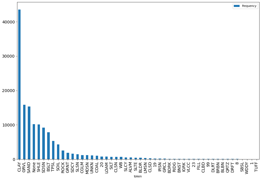
We saw in the previous post that the Namoi lithology logs data had their primary (major) lithology mostly completed. A substantial proportion had the label None nevertheless, despite descriptions that looked like they would obviously lead to a categorisation. There were many labels, with a long-tailed frequency histogram.

The aim of this post is (was) to get a classification training happening.

Spoiler alert: it won’t. Almost.

Rather than write a post after the fact pretending it was a totally smooth journey, the following walktrough deliberately keeps and highlights issues, albeit succinctly. Don’t jump to the conclusion that we will not get there eventually, or that Hugging Face is not good. When you adapt prior work to your own use case, you will likely stumble, so this post will make you feel in good company.

Kernel installation

The previous post was about data exploration and used mostly facilities such as pandas, not any deep learning related material. This post will, so we need to install Hugging Face. I did bump into a couple of issues while trying to get an environment going. I will not give the full grubby details, but highlight upfront a couple of things:

  • Do create a new dedicated conda environment for your work with Hugging Face, even if you already have an environment with e.g. pytorch you’d like to reuse.
  • The version 4.11.3 of HF transformers on the conda channel huggingface, at the time of writing, has a bug. You should install the packages from the conda-forge channel.

In a nutshell, for Linux:

myenv=hf
mamba create -n $myenv python=3.9 -c conda-forge
mamba install -n $myenv --yes ipykernel matplotlib sentencepiece scikit-learn -c conda-forge
mamba install -n $myenv --yes pytorch=1.11 -c pytorch -c nvidia -c conda-forge
mamba install -n $myenv --yes torchvision torchaudio -c pytorch -c nvidia -c conda-forge
mamba install -n $myenv --yes -c conda-forge datasets transformers
conda activate $myenv
python -m ipykernel install --user --name $myenv --display-name "Hugging Face"

and in Windows:

set myenv=hf
mamba create -n %myenv% python=3.9 -c conda-forge
mamba install -n %myenv% --yes ipykernel matplotlib sentencepiece scikit-learn -c conda-forge
mamba install -n %myenv% --yes pytorch=1.11 -c pytorch -c nvidia -c conda-forge
mamba install -n %myenv% --yes torchvision torchaudio -c pytorch -c nvidia -c conda-forge
mamba install -n %myenv% --yes -c conda-forge datasets transformers
conda activate %myenv%
python -m ipykernel install --user --name %myenv% --display-name "Hugging Face"

Walkthrough

Let’s get on with all the imports upfront (not obvious, mind you, but after the fact…)

import numpy as np
import pandas as pd
import torch
from datasets import Dataset
from transformers import AutoModelForSequenceClassification, AutoTokenizer
from pathlib import Path
from datasets import ClassLabel
from transformers import TrainingArguments, Trainer
from sklearn.metrics import f1_score
from collections import Counter

# Some column string identifiers
MAJOR_CODE = "MajorLithCode"
MAJOR_CODE_INT = "MajorLithoCodeInt"  # We will create a numeric representation of labels, which is (I think?) required by HF.
MINOR_CODE = "MinorLithCode"
DESC = "Description"
/home/abcdef/miniconda/envs/hf/lib/python3.9/site-packages/tqdm/auto.py:22: TqdmWarning: IProgress not found. Please update jupyter and ipywidgets. See https://ipywidgets.readthedocs.io/en/stable/user_install.html
  from .autonotebook import tqdm as notebook_tqdm
fn = Path("~").expanduser() / "data/ela/shp_namoi_river/NGIS_LithologyLog.csv"
litho_logs = pd.read_csv(
    fn, dtype={"FromDepth": str, "ToDepth": str, MAJOR_CODE: str, MINOR_CODE: str}
)

# To avoid importing from the ela package, copy a couple of functions:
# from ela.textproc import token_freq, plot_freq


def token_freq(tokens, n_most_common=50):
    list_most_common = Counter(tokens).most_common(n_most_common)
    return pd.DataFrame(list_most_common, columns=["token", "frequency"])


def plot_freq(dataframe, y_log=False, x="token", figsize=(15, 10), fontsize=14):
    """Plot a sorted histogram of work frequencies

    Args:
        dataframe (pandas dataframe): frequency of tokens, typically with colnames ["token","frequency"]
        y_log (bool): should there be a log scale on the y axis
        x (str): name of the columns with the tokens (i.e. words)
        figsize (tuple):
        fontsize (int):

    Returns:
        barplot: plot

    """
    p = dataframe.plot.bar(x=x, figsize=figsize, fontsize=fontsize)
    if y_log:
        p.set_yscale("log", nonposy="clip")
    return p


litho_classes = litho_logs[MAJOR_CODE].values
df_most_common = token_freq(litho_classes, 50)
plot_freq(df_most_common)
<AxesSubplot:xlabel='token'>

Imbalanced data sets

From the histogram above, it is pretty clear that labels are also not uniform an we have a class imbalance. Remember to skim Lithology classification using Hugging Face, part 1 for the initial data exploration if you have not done so already.

For the sake of the exercise in this post, I will reduce arbitrarily the number of labels used in this post, by just “forgetting” the less represented classes.

There are many resources about class imbalances. One of them is 8 Tactics to combat imbalanced classes in your machine learning dataset

Let’s see what labels we may want to keep for this post:

def sample_desc_for_code(major_code, n=50, seed=None):
    is_code = litho_logs[MAJOR_CODE] == major_code
    coded = litho_logs.loc[is_code][DESC]
    if seed is not None:
        np.random.seed(seed)
    return coded.sample(n=50)
sample_desc_for_code("UNKN", seed=123)
134145     (UNKNOWN), NO SAMPLE COLLECTED DUE TO WATER LOSS
134715    (UNKNOWN); COULD NOT BE LOGGED BECAUSE NO CUTT...
122303                                          GREY SHALEY
133856                                              NOMINAL
134378                                                 None
133542                                              DRILLER
122258                                        WATER BEARING
127916                                         WATER SUPPLY
133676                                              DRILLER
134399                                              DRILLER
134052                                              DRILLER
128031                         VERY SANDY STONES SOME LARGE
134140                                       SAMPLE MISSING
122282                              REDDISH YELLOW VOLCANIC
133623                                    WHITE CRYSTALLINE
134505                                              MISSING
133694                                              DRILLER
133585                                              DRILLER
134201                                              MISSING
134627                                              NO DATA
133816                                              DRILLER
133893                                              DRILLER
134232                                              DRILLER
133687                                              DRILLER
133871                                              DRILLER
133698                                              DRILLER
134752                                              MISSING
128077                           WATER BEARING WATER SUPPLY
122253                                         WATER SUPPLY
133607                                              DRILLER
133617                                              DRILLER
133643                                                 HARD
134526                                  (UNKNOWN) CORE LOSS
133709                                        SANDY STREAKS
123254                                 NOMINAL WATER SUPPLY
122219                                         WATER SUPPLY
133525                                              DRILLER
127799                                         WATER SUPPLY
133940                                              DRILLER
124775                              (UNKNOWN) WATER BEARING
126814                             (UNKNOWN); WATER BEARING
133965                                              DRILLER
134074                                              DRILLER
134395                                              DRILLER
133970                                              DRILLER
134262                                              DRILLER
122407                                         WATER SUPPLY
144370                                            S/S LT BR
125023                             (UNKNOWN); WATER BEARING
133675                                              DRILLER
Name: Description, dtype: object

The “unknown” category is rather interesting in fact, and worth keeping as a valid class.

Subsetting

Let’s keep “only” the main labels, for the sake of this exercise. We will remove None however, despite its potential interest. We will (hopefully) revisit this in another post.

labels_kept = df_most_common["token"][:17].values  # 17 first classes somewhat arbitraty
labels_kept = labels_kept[labels_kept != "None"]
labels_kept
array(['CLAY', 'GRVL', 'SAND', 'SHLE', 'SDSN', 'BSLT', 'TPSL', 'SOIL',
       'ROCK', 'GRNT', 'SDCY', 'SLSN', 'CGLM', 'MDSN', 'UNKN', 'COAL'],
      dtype=object)
kept = [x in labels_kept for x in litho_classes]
litho_logs_kept = litho_logs[kept].copy()  # avoid warning messages down the track.
litho_logs_kept.sample(10)
OBJECTID BoreID HydroCode RefElev RefElevDesc FromDepth ToDepth TopElev BottomElev MajorLithCode MinorLithCode Description Source LogType OgcFidTemp
70655 526412 10072593 GW031851.1.1 None UNK 53.94 59.13 None None CLAY NaN CLAY SANDY UNK 1 9308381
7173 64072 10043001 GW001815.1.1 None UNK 31.39 44.5 None None SHLE NaN SHALE UNK 1 8732384
30076 197788 10152523 GW099036.1.1 None UNK 181.0 228.0 None None SHLE NaN SHALE: GREY, FINE UNK 1 8870150
93967 701859 10105392 GW031140.1.1 None UNK 0.0 8.84 None None SOIL NaN SOIL CLAY UNK 1 9327759
115538 803595 10099300 GW970770.1.1 None UNK 36.6 38.1 None None SAND NaN SAND; FINE TO COARSE, BROWN UNK 1 9435886
107173 762000 10122945 GW018629.1.1 None UNK 72.54 74.37 None None SDSN NaN SANDSTONE YELLOW HARD UNK 1 9389679
106769 760370 10111007 GW026576.1.1 None UNK 65.23 71.32 None None SDSN NaN SANDSTONE WATER SUPPLY UNK 1 9388007
13553 114744 10116235 GW022175.1.1 None UNK 37.8 39.01 None None GRVL NaN GRAVEL FINE-COARSE UNK 1 8784472
142398 971715 10074454 GW901230.1.1 None UNK 20.0 24.0 None None GRVL NaN GRAVEL UNK 1 9567221
9664 85061 10043586 GW011521.1.1 None UNK 12.19 20.73 None None CLAY NaN CLAY YELLOW GRAVEL UNK 1 8753973
labels = ClassLabel(names=labels_kept)
int_labels = np.array([
    labels.str2int(x) for x in litho_logs_kept[MAJOR_CODE].values
])
int_labels = int_labels.astype(np.int8) # to mimick chapter3 HF so far as I can see
litho_logs_kept[MAJOR_CODE_INT] = int_labels

Class imbalance

Even our subset of 16 classes is rather imbalanced; the number of “clay” labels is looking more than 30 times that of “coal” just by eyeballing.

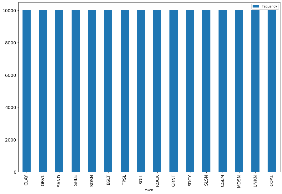
The post by Jason Brownlee 8 Tactics to Combat Imbalanced Classes in Your Machine Learning Dataset, outlines several approaches. One of them is to resample from labels, perhaps with replacement, to equalise classes. It is a relatively easy approach to implement, but there are issues, growing with the level of imbalance. Notably, if too many rows from underrepresented classes are repeated, there is an increased tendency to overfitting at training.

The video Simple Training with the 🤗 Transformers Trainer (at 669 seconds) also explains the issues with imbalances and crude resampling. It offers instead a solution with class weighting that is more robust. That approach is evoked in Jason’s post, but the video has a “Hugging Face style” implementation ready to repurpose.

Resample with replacement

Just for information, what we’d do with a relatively crude resampling may be:

def sample_major_lithocode(dframe, code, n=10000, seed=None):
    x = dframe[dframe[MAJOR_CODE] == code]
    replace = n > len(x)
    return x.sample(n=n, replace=replace, random_state=seed)
sample_major_lithocode(litho_logs_kept, "CLAY", n=10, seed=0)
OBJECTID BoreID HydroCode RefElev RefElevDesc FromDepth ToDepth TopElev BottomElev MajorLithCode MinorLithCode Description Source LogType OgcFidTemp MajorLithoCodeInt
106742 760246 10144429 GW030307.1.1 279.5 NGS 54.3 72.2 225.2 207.3 CLAY NaN CLAY LIGHT BROWN GRAVEL UNK 1 9387877 0
138850 950521 10147004 GW036015.2.2 236.0 NGS 73.15 74.676 162.85 161.324 CLAY NaN CLAY; AS ABOVE, MORE MICACEOUS & FINE GRAVEL (... ?? - WC&IC 2 9543085 0
30006 197243 10049338 GW062392.1.1 None UNK 63.0 64.0 None None CLAY NaN CLAY SANDY UNK 1 8869540 0
3225 29304 10142901 GW014623.1.1 None UNK 22.86 23.47 None None CLAY NaN CLAY SANDY UNK 1 8696556 0
9795 86262 10121680 GW009977.1.1 None UNK 39.01 42.67 None None CLAY NaN CLAY YELLOW PUGGY UNK 1 8755205 0
49588 427460 10067562 GW964964.1.1 None UNK 11.0 14.0 None None CLAY NaN CLAY UNK 1 9199868 0
136116 943202 10055892 GW971627.1.1 None UNK 14.0 20.0 None None CLAY NaN GREY WET CLAY UNK 1 9534634 0
5723 50788 10049974 GW010017.1.1 None UNK 14.02 24.38 None None CLAY NaN CLAY RED SANDY UNK 1 8718677 0
94938 706287 10018922 GW022845.1.1 None UNK 1.22 11.58 None None CLAY NaN CLAY UNK 1 9332267 0
38277 287347 10132392 GW042735.1.1 None UNK 0.75 6.0 None None CLAY NaN CLAY UNK 1 8942094 0
balanced_litho_logs = [
    sample_major_lithocode(litho_logs_kept, code, n=10000, seed=0)
    for code in labels_kept
]
balanced_litho_logs = pd.concat(balanced_litho_logs)
balanced_litho_logs.head()
OBJECTID BoreID HydroCode RefElev RefElevDesc FromDepth ToDepth TopElev BottomElev MajorLithCode MinorLithCode Description Source LogType OgcFidTemp MajorLithoCodeInt
106742 760246 10144429 GW030307.1.1 279.5 NGS 54.3 72.2 225.2 207.3 CLAY NaN CLAY LIGHT BROWN GRAVEL UNK 1 9387877 0
138850 950521 10147004 GW036015.2.2 236.0 NGS 73.15 74.676 162.85 161.324 CLAY NaN CLAY; AS ABOVE, MORE MICACEOUS & FINE GRAVEL (... ?? - WC&IC 2 9543085 0
30006 197243 10049338 GW062392.1.1 None UNK 63.0 64.0 None None CLAY NaN CLAY SANDY UNK 1 8869540 0
3225 29304 10142901 GW014623.1.1 None UNK 22.86 23.47 None None CLAY NaN CLAY SANDY UNK 1 8696556 0
9795 86262 10121680 GW009977.1.1 None UNK 39.01 42.67 None None CLAY NaN CLAY YELLOW PUGGY UNK 1 8755205 0
plot_freq(token_freq(balanced_litho_logs[MAJOR_CODE].values, 50))
<AxesSubplot:xlabel='token'>

Dealing with imbalanced classes with weights

Instead of the resampling above, we adapt the approach creating weights for the Trainer we will run.

sorted_counts = litho_logs_kept[MAJOR_CODE].value_counts()
sorted_counts
CLAY    43526
GRVL    15824
SAND    15317
SHLE    10158
SDSN     9199
BSLT     7894
TPSL     5300
SOIL     4347
ROCK     2549
GRNT     1852
SDCY     1643
SLSN     1443
CGLM     1233
MDSN     1207
UNKN     1125
COAL     1040
Name: MajorLithCode, dtype: int64
sorted_counts / sorted_counts.sum()
CLAY    0.351990
GRVL    0.127967
SAND    0.123867
SHLE    0.082147
SDSN    0.074391
BSLT    0.063838
TPSL    0.042860
SOIL    0.035154
ROCK    0.020613
GRNT    0.014977
SDCY    0.013287
SLSN    0.011669
CGLM    0.009971
MDSN    0.009761
UNKN    0.009098
COAL    0.008410
Name: MajorLithCode, dtype: float64
class_weights = (1 - sorted_counts / sorted_counts.sum()).values
class_weights
array([0.64801022, 0.87203312, 0.87613317, 0.91785342, 0.92560874,
       0.93616213, 0.95713951, 0.96484631, 0.97938653, 0.98502309,
       0.98671325, 0.98833062, 0.99002887, 0.99023913, 0.99090225,
       0.99158964])

We check that cuda is available (of course optional)

assert torch.cuda.is_available()

On Linux if you have a DELL laptop with an NVIDIA card, but nvidia-smi returns: NVIDIA-SMI has failed because it couldn't communicate with the NVIDIA driver. Make sure that the latest NVIDIA driver is installed and running, you may need to change your kernel specification file $HOME/.local/share/jupyter/kernels/hf/kernel.json. This behavior seems to depend on the version of Linux kernel you have. It certainly changed out of the blue for me from yesterday, despite no change that I can tell.

optirun nvidia-smi returning a proper graphic card report should be a telltale sign you have to update your kernel.json like so:

{
 "argv": [
  "optirun",
  "/home/your_ident/miniconda/envs/hf/bin/python",
  "-m",
  "ipykernel_launcher",
  "-f",
  "{connection_file}"
 ],
 "display_name": "Hugging Face",
 "language": "python",
 "metadata": {
  "debugger": true
 }
}

You may need to restart jupyter-lab, or visual studio code, etc., for change to take effect. Restarting the kernel may not be enough, conter-intuitively.

Background details about optirun architecture at [Bumblebee Debian]https://wiki.debian.org/Bumblebee

class_weights = torch.from_numpy(class_weights).float().to("cuda")
class_weights
tensor([0.6480, 0.8720, 0.8761, 0.9179, 0.9256, 0.9362, 0.9571, 0.9648, 0.9794,
        0.9850, 0.9867, 0.9883, 0.9900, 0.9902, 0.9909, 0.9916],
       device='cuda:0')
model_nm = "microsoft/deberta-v3-small"

Tokenisation

Bump on the road; download operations taking too long

At this point I spent more hours than I wish I had on an issue, perhaps very unusual.

The operation tokz = AutoTokenizer.from_pretrained(model_nm) was taking an awful long time to complete:

CPU times: user 504 ms, sys: 57.9 ms, total: 562 ms
Wall time: 14min 13s

To cut a long story short, I managed to figure out what was going on. It is documented on the Hugging Face forum at: Some HF operations take an excessively long time to complete. If you have issues where HF operations take a long time, read it.

Now back to the tokenisation story. Note that the local caching may be superflous if you do not encounter the issue just mentioned.

max_length = 128
p = Path("./tokz_pretrained")
pretrained_model_name_or_path = p if p.exists() else model_nm
# https://discuss.huggingface.co/t/sentence-transformers-paraphrase-minilm-fine-tuning-error/9612/4
tokz = AutoTokenizer.from_pretrained(pretrained_model_name_or_path, use_fast=True, max_length=max_length, model_max_length=max_length)
if not p.exists():
    tokz.save_pretrained("./tokz_pretrained")

Let’s see what this does on a typical lithology description

tokz.tokenize("CLAY, VERY SANDY")
['▁C', 'LAY', ',', '▁VERY', '▁S', 'ANDY']

Well, the vocabulary is probably case sensitive and all the descriptions being uppercase in the source data are likely problematic. Let’s check what happens on lowercase descriptions:

tokz.tokenize("clay, very sandy")
['▁clay', ',', '▁very', '▁sandy']

This looks better. So let’s change the descriptions to lowercase; we are not loosing any relevent information in this case, I think.

# note: no warnings because we used .copy() earlier to create litho_logs_kept
litho_logs_kept[DESC] = litho_logs_kept[DESC].str.lower()
litho_logs_kept_mini = litho_logs_kept[[MAJOR_CODE_INT, DESC]]
litho_logs_kept_mini.sample(n=10)
MajorLithoCodeInt Description
8256 5 basalt
96820 4 sandstone
36776 2 sand
110231 0 clay; light brown, very silty
80270 1 gravel & large stones
17592 1 gravel water supply
74437 0 clay
22904 5 basalt stones
71578 1 gravel very clayey water supply
73030 3 shale

Create dataset and tokenisation

We want to create a dataset such that tokenised data is of uniform shape (better for running on GPU) Applying the technique in this segment of the HF course video. Cheating a bit on guessing the length (I know from offline checks that max is 90 tokens)

ds = Dataset.from_pandas(litho_logs_kept_mini)

def tok_func(x):
    return tokz(
        x[DESC],
        padding="max_length",
        truncation=True,
        max_length=max_length,
        return_tensors="pt",
    )

The Youtube video above suggests to use tok_ds = ds.map(tok_func, batched=True) for a faster execution; however I ended up with the foollowing error:

TypeError: Provided `function` which is applied to all elements of table returns a `dict` of types [<class 'torch.Tensor'>, <class 'torch.Tensor'>, <class 'torch.Tensor'>]. When using `batched=True`, make sure provided `function` returns a `dict` of types like `(<class 'list'>, <class 'numpy.ndarray'>)`.

The following non-batched option works in a reasonable time:

tok_ds = ds.map(tok_func)
Parameter 'function'=<function tok_func at 0x7f0d047695e0> of the transform datasets.arrow_dataset.Dataset._map_single couldn't be hashed properly, a random hash was used instead. Make sure your transforms and parameters are serializable with pickle or dill for the dataset fingerprinting and caching to work. If you reuse this transform, the caching mechanism will consider it to be different from the previous calls and recompute everything. This warning is only showed once. Subsequent hashing failures won't be showed.
100%|████████████████████████████████████████████████████████████████████████████████████████████████████████████████████████████████████████████| 123657/123657 [00:24<00:00, 4962.06ex/s]
tok_ds_tmp = tok_ds[:5]
tok_ds_tmp.keys()
dict_keys(['MajorLithoCodeInt', 'Description', '__index_level_0__', 'input_ids', 'token_type_ids', 'attention_mask'])
# check the length of vectors is indeed 128:
len(tok_ds_tmp["input_ids"][0][0])
128
num_labels = len(labels_kept)
# NOTE: the local caching may be superflous
p = Path("./model_pretrained")

model_name = p if p.exists() else model_nm
model = AutoModelForSequenceClassification.from_pretrained(model_name, num_labels=num_labels, max_length=max_length)
                                                           # label2id=label2id, id2label=id2label).to(device) 
if not p.exists():
    model.save_pretrained(p)
print(type(model))
<class 'transformers.models.deberta_v2.modeling_deberta_v2.DebertaV2ForSequenceClassification'>
# Different approach, but one that I am not sure how to progress to a hugging face Dataset. Borrowed from [this video](https://youtu.be/1pedAIvTWXk?list=PLo2EIpI_JMQvWfQndUesu0nPBAtZ9gP1o&t=143)
# litho_desc_list = [x for x in litho_logs_kept_mini[DESC].values]
# input_descriptions = tokz(litho_desc_list, padding=True, truncation=True, max_length=256, return_tensors='pt')
# input_descriptions['input_ids'].shape
# model(input_descriptions['input_ids'][:5,:], attention_mask=input_descriptions['attention_mask'][:5,:]).logits
tok_ds
Dataset({
    features: ['MajorLithoCodeInt', 'Description', '__index_level_0__', 'input_ids', 'token_type_ids', 'attention_mask'],
    num_rows: 123657
})

Transformers always assumes that your labels has the column name “labels”. Odd, but at least this fosters a consistent system, so why not:

tok_ds = tok_ds.rename_columns({MAJOR_CODE_INT: "labels"})
tok_ds = tok_ds.remove_columns(['Description', '__index_level_0__'])
# We want to make sure we work on the GPU, so at least make sure we have torch tensors.
# Note that HF is supposed to take care of movind data to the GPU if available, so you should not ahve to manually copy the data to the GPU device
tok_ds.set_format("torch")
# args = TrainingArguments(output_dir='./litho_outputs', learning_rate=lr, warmup_ratio=0.1, lr_scheduler_type='cosine', fp16=True,
#     evaluation_strategy="epoch", per_device_train_batch_size=bs, per_device_eval_batch_size=bs*2,
#     num_train_epochs=epochs, weight_decay=0.01, report_to='none')
dds = tok_ds.train_test_split(0.25, seed=42)
dds.keys()
dict_keys(['train', 'test'])
tok_ds.features['labels'] = labels
tok_ds.features

# TODO:
#     This differs from chapter3 of HF course https://huggingface.co/course/chapter3/4?fw=pt    
# {'attention_mask': Sequence(feature=Value(dtype='int8', id=None), length=-1, id=None),
#  'input_ids': Sequence(feature=Value(dtype='int32', id=None), length=-1, id=None),
#  'labels': ClassLabel(num_classes=2, names=['not_equivalent', 'equivalent'], id=None),
#  'token_type_ids': Sequence(feature=Value(dtype='int8', id=None), length=-1, id=None)}
{'labels': ClassLabel(num_classes=16, names=array(['CLAY', 'GRVL', 'SAND', 'SHLE', 'SDSN', 'BSLT', 'TPSL', 'SOIL',
        'ROCK', 'GRNT', 'SDCY', 'SLSN', 'CGLM', 'MDSN', 'UNKN', 'COAL'],
       dtype=object), id=None),
 'input_ids': Sequence(feature=Sequence(feature=Value(dtype='int32', id=None), length=-1, id=None), length=-1, id=None),
 'token_type_ids': Sequence(feature=Sequence(feature=Value(dtype='int8', id=None), length=-1, id=None), length=-1, id=None),
 'attention_mask': Sequence(feature=Sequence(feature=Value(dtype='int8', id=None), length=-1, id=None), length=-1, id=None)}
tok_ds['input_ids'][0]
[tensor([    1,  3592, 14432,  8076,     2,     0,     0,     0,     0,     0,
             0,     0,     0,     0,     0,     0,     0,     0,     0,     0,
             0,     0,     0,     0,     0,     0,     0,     0,     0,     0,
             0,     0,     0,     0,     0,     0,     0,     0,     0,     0,
             0,     0,     0,     0,     0,     0,     0,     0,     0,     0,
             0,     0,     0,     0,     0,     0,     0,     0,     0,     0,
             0,     0,     0,     0,     0,     0,     0,     0,     0,     0,
             0,     0,     0,     0,     0,     0,     0,     0,     0,     0,
             0,     0,     0,     0,     0,     0,     0,     0,     0,     0,
             0,     0,     0,     0,     0,     0,     0,     0,     0,     0,
             0,     0,     0,     0,     0,     0,     0,     0,     0,     0,
             0,     0,     0,     0,     0,     0,     0,     0,     0,     0,
             0,     0,     0,     0,     0,     0,     0,     0])]
# https://huggingface.co/docs/transformers/training
# from Jeremy's notebook:
# def compute_metrics(eval_pred):
#     logits, labels = eval_pred
#     predictions = np.argmax(logits, axis=-1)
#     return metric.compute(predictions=predictions, references=labels)
# Defining the Trainer to compute Custom Loss Function, adapted from [Simple Training with the 🤗 Transformers Trainer, around 840 seconds](https://youtu.be/u--UVvH-LIQ?t=840)
class WeightedLossTrainer(Trainer):
    def compute_loss(self, model, inputs, return_outputs=False):
        # Feed inputs to model and extract logits
        outputs = model(**inputs)
        logits = outputs.get("logits")
        # Extract Labels
        labels = inputs.get("labels")
        # Define loss function with class weights
        loss_func = torch.nn.CrossEntropyLoss(weight=class_weights)
        # Compute loss
        loss = loss_func(logits, labels)
        return (loss, outputs) if return_outputs else loss
def compute_metrics(eval_pred):
    labels = eval_pred.label_ids
    predictions = eval_pred.predictions.argmax(-1)
    f1 = f1_score(labels, predictions, average="weighted")
    return {"f1": f1}
output_dir = "./hf_training"
batch_size = 64 # 128
epochs = 5
lr = 8e-5
training_args = TrainingArguments(
    output_dir=output_dir,
    num_train_epochs=epochs,
    learning_rate=lr,
    lr_scheduler_type="cosine",
    per_device_train_batch_size=batch_size,
    per_device_eval_batch_size=batch_size * 2,
    weight_decay=0.01,
    evaluation_strategy="epoch",
    logging_steps=len(dds["train"]),
    fp16=True,
    push_to_hub=False,
    report_to="none",
)
model = model.to("cuda:0")

The above nay not be strictly necessary, depending on your version of transformers. I bumped into the following issue, which was probably the transformers 4.11.3 bug: RuntimeError: Expected all tensors to be on the same device, but found at least two devices, cuda:0 and cpu! (when checking argument for argument index in method wrapper__index_select)

trainer = Trainer(
    model=model,
    args=training_args,
    train_dataset=dds["train"],
    eval_dataset=dds["test"],
    tokenizer=tokz,
    compute_metrics=compute_metrics,
)
Using amp half precision backend

Training?

You did read the introduction and its spoiler alert, right?

trainer.train()
/home/abcdef/miniconda/envs/hf/lib/python3.9/site-packages/transformers/optimization.py:306: FutureWarning: This implementation of AdamW is deprecated and will be removed in a future version. Use the PyTorch implementation torch.optim.AdamW instead, or set `no_deprecation_warning=True` to disable this warning
  warnings.warn(
***** Running training *****
  Num examples = 92742
  Num Epochs = 5
  Instantaneous batch size per device = 64
  Total train batch size (w. parallel, distributed & accumulation) = 64
  Gradient Accumulation steps = 1
  Total optimization steps = 7250
RuntimeError: The size of tensor a (768) must match the size of tensor b (128) at non-singleton dimension 3

Stocktake and conclusion

So, as announced at the start of this post, we hit a pothole in our journey.

RuntimeError: The size of tensor a (768) must match the size of tensor b (128) at non-singleton dimension 3

Where the number (768) comes from is a bit of a mystery. I gather from Googling that this may have to do with the embedding of the Deberta model we are trying to fine tune, but I may be off the mark.

It is probably something at which an experience NLP practitioner will roll their eyes.

That’s OK, We’ll get there.